Algorithmic Stability and Learning Theory

Algorithmic Stability and Learning Theory

Learning Objectives

By the end of this article, you will: 1. Understand what algorithmic stability means and why it matters 2. Learn different types of stability measures 3. See how stability affects model generalization 4. Practice implementing stability checks 5. Learn best practices for developing stable models

Introduction

Imagine building a house of cards . If a slight breeze can topple it, we’d say it’s unstable. Similarly, in machine learning, we want our models to be stable - small changes in the training data shouldn’t cause dramatic changes in predictions.

import numpy as np
import matplotlib.pyplot as plt
import seaborn as sns
from sklearn.linear_model import Ridge
from sklearn.preprocessing import StandardScaler

# Set random seed for reproducibility
np.random.seed(42)

1. Understanding Stability Through Examples

Let’s visualize what stability means with a simple example:

def generate_data(n_samples=100):
    X = np.linspace(0, 10, n_samples).reshape(-1, 1)
    y = 0.5 * X.ravel() + np.sin(X.ravel()) + np.random.normal(0, 0.1, n_samples)
    return X, y

def plot_stability_comparison(alpha1=0.1, alpha2=10.0):
    X, y = generate_data()
    
    # Create two models with different regularization
    model1 = Ridge(alpha=alpha1)
    model2 = Ridge(alpha=alpha2)
    
    # Fit models
    model1.fit(X, y)
    model2.fit(X, y)
    
    # Generate predictions
    X_test = np.linspace(0, 10, 200).reshape(-1, 1)
    y_pred1 = model1.predict(X_test)
    y_pred2 = model2.predict(X_test)
    
    # Plot results
    plt.figure(figsize=(12, 6))
    plt.scatter(X, y, color='blue', alpha=0.5, label='Data points')
    plt.plot(X_test, y_pred1, 'r-', label=f'Less stable (α={alpha1})')
    plt.plot(X_test, y_pred2, 'g-', label=f'More stable (α={alpha2})')
    plt.title('Stability Comparison: Effect of Regularization')
    plt.xlabel('X')
    plt.ylabel('y')
    plt.legend()
    plt.show()

plot_stability_comparison()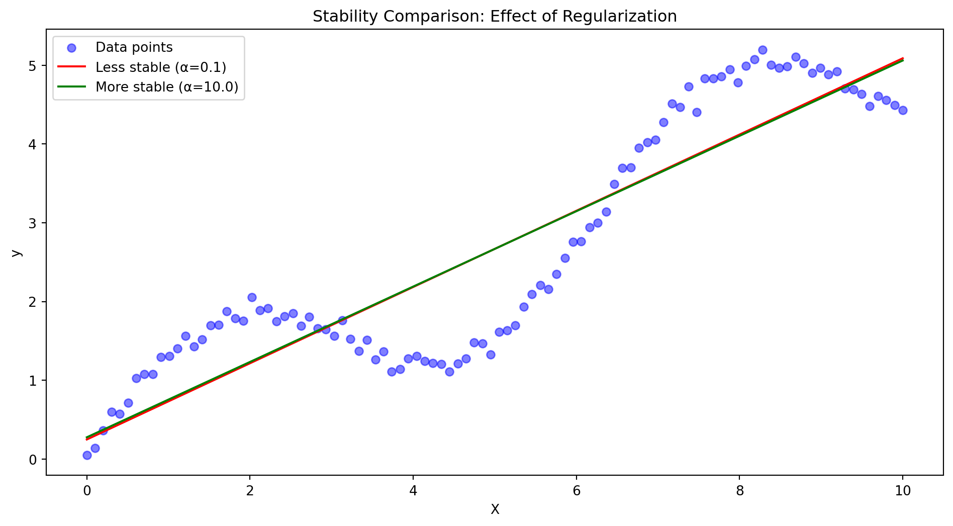

Key Insight

Notice how the more stable model (green line) is less sensitive to individual data points, while the less stable model (red line) overfits to the noise in the data.

Fundamental Concepts

1. Stability Definitions

Hypothesis stability:

\[ |\ell(A_S,z) - \ell(A_{S^i},z)| \leq \beta_m \]

Where: - \(A_S\) is algorithm output on dataset \(S\) - \(S^i\) is dataset with i-th example replaced - \(\beta_m\) is stability coefficient

Uniform stability:

\[ \sup_{S,z,i}|\ell(A_S,z) - \ell(A_{S^i},z)| \leq \beta \]

2. Loss Stability

Point-wise loss stability:

\[ |\ell(h_S,z) - \ell(h_{S^i},z)| \leq \beta \]

Average loss stability:

\[ |\mathbb{E}_{z \sim \mathcal{D}}[\ell(h_S,z) - \ell(h_{S^i},z)]| \leq \beta \]

3. Generalization Bounds

McDiarmid’s inequality based bound:

\[ P(|R(A_S) - \hat{R}_S(A_S)| > \epsilon) \leq 2\exp(-\frac{2m\epsilon^2}{(4\beta)^2}) \]

Expected generalization error:

\[ |\mathbb{E}[R(A_S) - \hat{R}_S(A_S)]| \leq \beta \]

Types of Stability

1. Strong Stability

Definition:

\[ \sup_{S,S': |S \triangle S'| = 2}\|A_S - A_{S'}\| \leq \beta_m \]

Generalization bound:

\[ P(|R(A_S) - \hat{R}_S(A_S)| > \epsilon) \leq 2\exp(-\frac{m\epsilon^2}{2\beta_m^2}) \]

2. Cross-Validation Stability

Leave-one-out stability:

\[ |\mathbb{E}_{S,z}[\ell(A_S,z) - \ell(A_{S^{-i}},z)]| \leq \beta_m \]

k-fold stability:

\[ |\mathbb{E}_{S,z}[\ell(A_S,z) - \ell(A_{S_k},z)]| \leq \beta_m \]

3. Algorithmic Robustness

\((K,\epsilon(\cdot))\)-robustness:

\[ P_{S,z}(|\ell(A_S,z) - \ell(A_S,z')| > \epsilon(m)) \leq K/m \]

Where: - \(z,z'\) are in same partition - \(K\) is number of partitions - \(\epsilon(m)\) is robustness parameter

Stability Analysis

1. Regularization and Stability

Tikhonov regularization:

\[ A_S = \arg\min_{h \in \mathcal{H}} \frac{1}{m}\sum_{i=1}^m \ell(h,z_i) + \lambda\|h\|^2 \]

Stability bound:

\[ \beta \leq \frac{L^2}{2m\lambda} \]

Where: - \(L\) is Lipschitz constant - \(\lambda\) is regularization parameter

2. Gradient Methods

Gradient descent stability:

\[ \|w_t - w_t'\| \leq (1+\eta L)^t\|w_0 - w_0'\| \]

SGD stability:

\[ \mathbb{E}[\|w_t - w_t'\|^2] \leq \frac{\eta^2L^2}{2m} \]

3. Ensemble Methods

Bagging stability:

\[ \beta_{\text{bag}} \leq \frac{\beta}{\sqrt{B}} \]

Where: - \(B\) is number of bootstrap samples - \(\beta\) is base learner stability

Practical Stability Analysis

Let’s implement some stability measures and visualize them:

class StabilityAnalyzer:
    def __init__(self, model_class, **model_params):
        self.model_class = model_class
        self.model_params = model_params
        
    def measure_hypothesis_stability(self, X, y, n_perturbations=10):
        """Measure hypothesis stability by perturbing data points"""
        m = len(X)
        stabilities = []
        
        # Original model
        base_model = self.model_class(**self.model_params)
        base_model.fit(X, y)
        base_preds = base_model.predict(X)
        
        for _ in range(n_perturbations):
            # Randomly replace one point
            idx = np.random.randint(m)
            X_perturbed = X.copy()
            y_perturbed = y.copy()
            
            # Add small noise to selected point
            X_perturbed[idx] += np.random.normal(0, 0.1, X.shape[1])
            
            # Train perturbed model
            perturbed_model = self.model_class(**self.model_params)
            perturbed_model.fit(X_perturbed, y_perturbed)
            perturbed_preds = perturbed_model.predict(X)
            
            # Calculate stability measure
            stability = np.mean(np.abs(base_preds - perturbed_preds))
            stabilities.append(stability)
            
        return np.mean(stabilities), np.std(stabilities)

# Example usage with Ridge Regression
def compare_model_stability():
    # Generate synthetic data
    np.random.seed(42)
    X = np.random.randn(100, 2)
    y = 0.5 * X[:, 0] + 0.3 * X[:, 1] + np.random.normal(0, 0.1, 100)
    
    # Compare stability with different regularization strengths
    alphas = [0.01, 0.1, 1.0, 10.0]
    stabilities = []
    errors = []
    
    for alpha in alphas:
        analyzer = StabilityAnalyzer(Ridge, alpha=alpha)
        stability, error = analyzer.measure_hypothesis_stability(X, y)
        stabilities.append(stability)
        errors.append(error)
    
    # Plot results
    plt.figure(figsize=(10, 6))
    plt.errorbar(alphas, stabilities, yerr=errors, fmt='o-', capsize=5)
    plt.xscale('log')
    plt.xlabel('Regularization Strength (α)')
    plt.ylabel('Stability Measure')
    plt.title('Model Stability vs Regularization')
    plt.grid(True, alpha=0.3)
    plt.show()

compare_model_stability()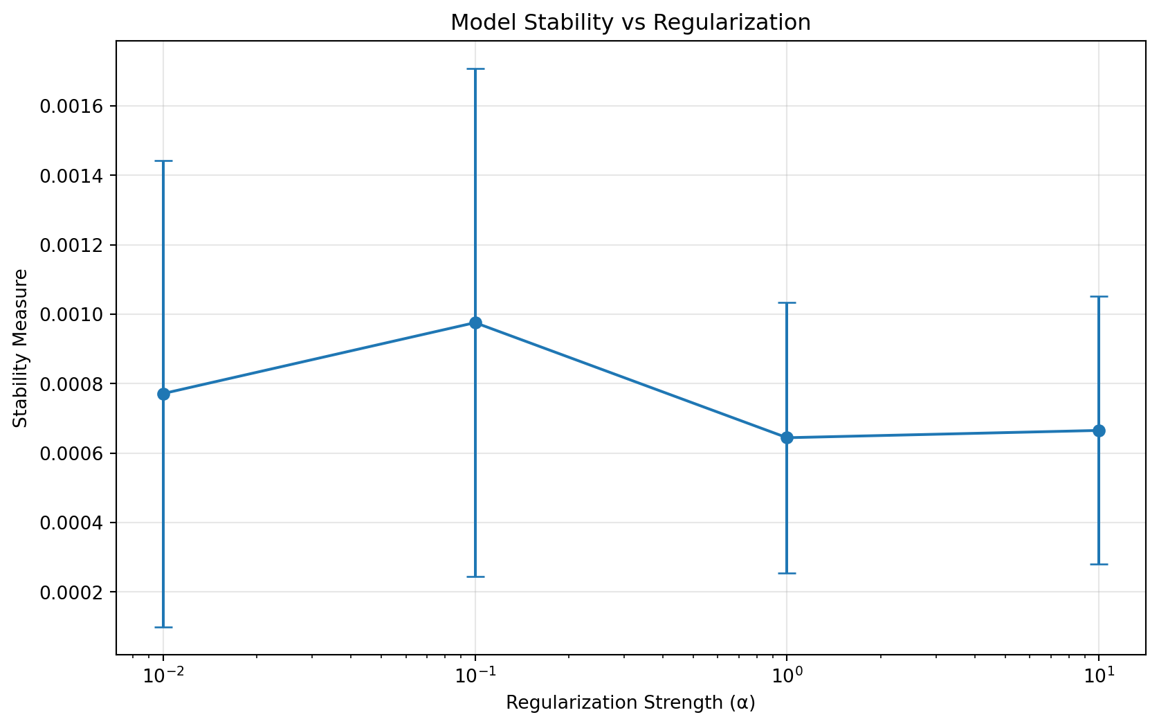

Interpreting Stability Results

Lower values indicate more stable models. Notice how increasing regularization generally improves stability.

Cross-Validation Stability

Let’s visualize how different cross-validation strategies affect stability:

def analyze_cv_stability(n_splits=[2, 5, 10], n_repeats=10):
    """Analyze stability across different CV splits"""
    from sklearn.model_selection import KFold
    
    # Generate data
    X = np.random.randn(200, 2)
    y = 0.5 * X[:, 0] + 0.3 * X[:, 1] + np.random.normal(0, 0.1, 200)
    
    results = {k: [] for k in n_splits}
    
    for k in n_splits:
        for _ in range(n_repeats):
            # Create k-fold split
            kf = KFold(n_splits=k, shuffle=True)
            fold_scores = []
            
            for train_idx, val_idx in kf.split(X):
                # Train model
                model = Ridge(alpha=1.0)
                model.fit(X[train_idx], y[train_idx])
                
                # Get score
                score = model.score(X[val_idx], y[val_idx])
                fold_scores.append(score)
            
            # Calculate stability of scores
            results[k].append(np.std(fold_scores))
    
    # Plot results
    plt.figure(figsize=(10, 6))
    plt.boxplot([results[k] for k in n_splits], labels=[f'{k}-fold' for k in n_splits])
    plt.ylabel('Score Stability (std)')
    plt.xlabel('Cross-Validation Strategy')
    plt.title('Cross-Validation Stability Analysis')
    plt.grid(True, alpha=0.3)
    plt.show()

analyze_cv_stability()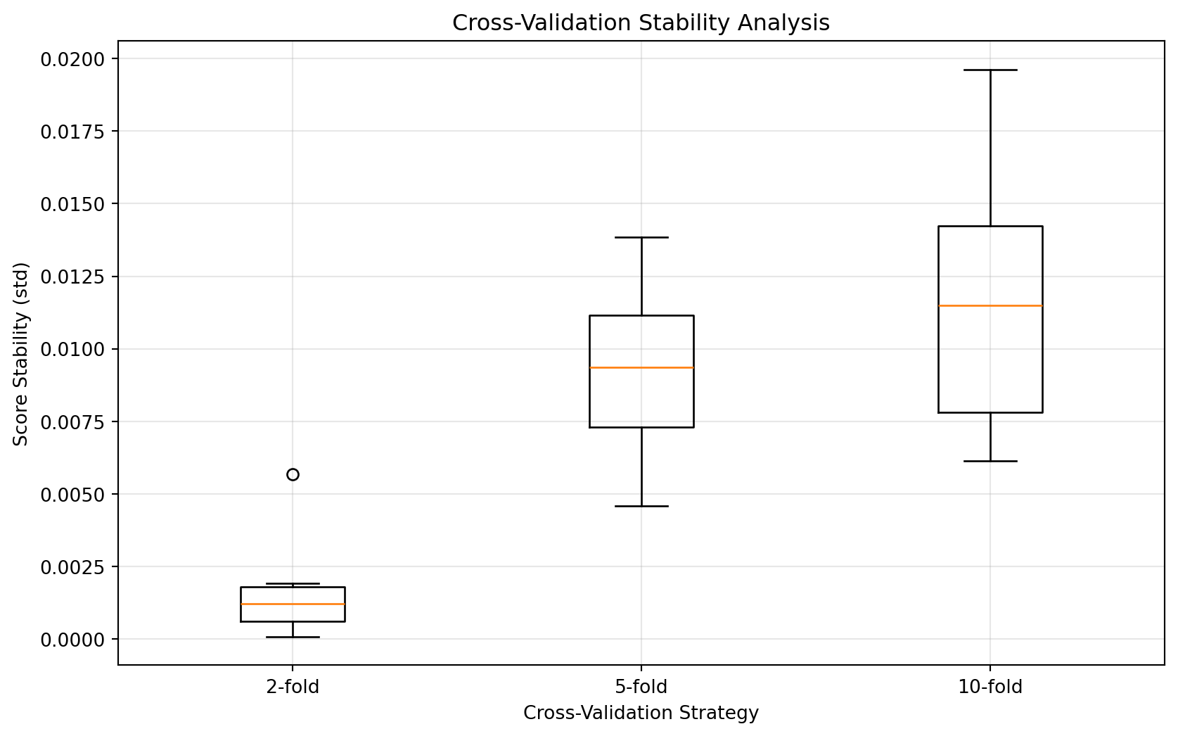

Cross-Validation Insight

More folds generally lead to more stable results but require more computational resources.

Ensemble Stability

Let’s implement and visualize the stability of ensemble methods:

def analyze_ensemble_stability(n_estimators=[1, 5, 10, 20]):
    """Analyze how ensemble size affects stability"""
    from sklearn.ensemble import BaggingRegressor
    
    # Generate data
    X = np.random.randn(150, 2)
    y = 0.5 * X[:, 0] + 0.3 * X[:, 1] + np.random.normal(0, 0.1, 150)
    
    # Test data for stability measurement
    X_test = np.random.randn(50, 2)
    
    stabilities = []
    errors = []
    
    for n in n_estimators:
        # Create multiple ensembles with same size
        predictions = []
        for _ in range(10):
            model = BaggingRegressor(
                estimator=Ridge(alpha=1.0),
                n_estimators=n,
                random_state=None
            )
            model.fit(X, y)
            predictions.append(model.predict(X_test))
        
        # Calculate stability across different ensemble instances
        stability = np.mean([np.std(pred) for pred in zip(*predictions)])
        error = np.std([np.std(pred) for pred in zip(*predictions)])
        
        stabilities.append(stability)
        errors.append(error)
    
    # Plot results
    plt.figure(figsize=(10, 6))
    plt.errorbar(n_estimators, stabilities, yerr=errors, fmt='o-', capsize=5)
    plt.xlabel('Number of Estimators')
    plt.ylabel('Prediction Stability')
    plt.title('Ensemble Size vs. Prediction Stability')
    plt.grid(True, alpha=0.3)
    plt.show()

analyze_ensemble_stability()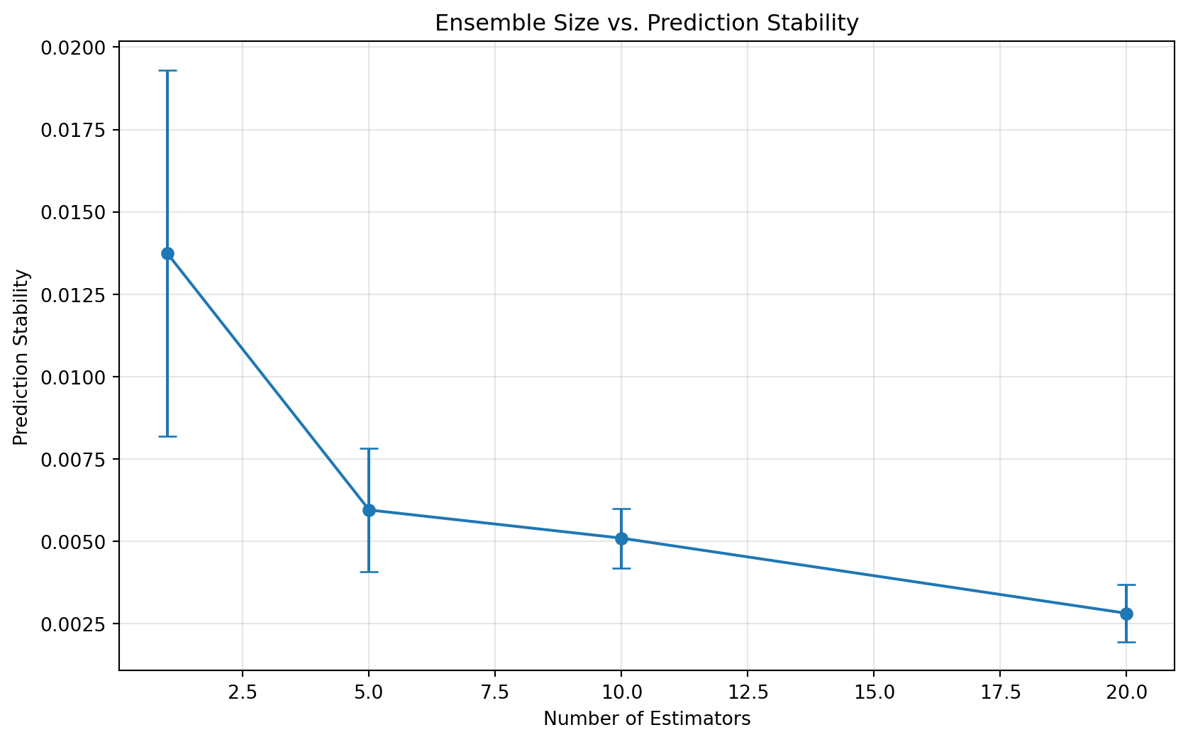

Ensemble Benefits

Larger ensembles tend to have more stable predictions, demonstrating the “wisdom of crowds” effect.

Applications

1. Regularized Learning

Ridge regression stability:

\[ \beta_{\text{ridge}} \leq \frac{4M^2}{m\lambda} \]

Where: - \(M\) is bound on features - \(\lambda\) is regularization

2. Online Learning

Online stability:

\[ \mathbb{E}[\|w_t - w_t'\|] \leq \frac{2G}{\lambda\sqrt{t}} \]

Where: - \(G\) is gradient bound - \(t\) is iteration number

3. Deep Learning

Dropout stability:

\[ \beta_{\text{dropout}} \leq \frac{p(1-p)L^2}{m} \]

Where: - \(p\) is dropout probability - \(L\) is network Lipschitz constant

Advanced Topics

1. Local Stability

Definition:

\[ |\ell(A_S,z) - \ell(A_{S^i},z)| \leq \beta(z) \]

Adaptive bound:

\[ P(|R(A_S) - \hat{R}_S(A_S)| > \epsilon) \leq 2\exp(-\frac{2m\epsilon^2}{\mathbb{E}[\beta(Z)^2]}) \]

2. Distribution Stability

Definition:

\[ \|\mathcal{D}_{A_S} - \mathcal{D}_{A_{S^i}}\|_1 \leq \beta \]

Generalization:

\[ |\mathbb{E}[R(A_S)] - \mathbb{E}[\hat{R}_S(A_S)]| \leq \beta \]

3. Algorithmic Privacy

Differential privacy:

\[ P(A_S \in E) \leq e^\epsilon P(A_{S'} \in E) \]

Privacy-stability relationship:

\[ \beta \leq \epsilon L \]

Theoretical Results

1. Stability Hierarchy

Relationships:

\[ \text{Uniform} \implies \text{Hypothesis} \implies \text{Point-wise} \implies \text{Average} \]

Equivalence conditions:

\[ \beta_{\text{uniform}} = \beta_{\text{hypothesis}} \iff \text{convex loss} \]

2. Lower Bounds

Minimal stability:

\[ \beta_m \geq \Omega(\frac{1}{\sqrt{m}}) \]

Optimal rates:

\[ \beta_m = \Theta(\frac{1}{m}) \]

3. Composition Theorems

Serial composition:

\[ \beta_{A \circ B} \leq \beta_A + \beta_B \]

Parallel composition:

\[ \beta_{\text{parallel}} \leq \max_i \beta_i \]

Implementation Considerations

1. Algorithm Design

1. Regularization:
   • Choose appropriate \(\lambda\)
   • Balance stability-accuracy
   • Adaptive regularization
2. Optimization:
   • Step size selection
   • Batch size impact
   • Momentum effects
3. Architecture:
   • Layer stability
   • Skip connections
   • Normalization impact

2. Stability Measures

1. Empirical Stability:
   • Leave-one-out estimates
   • Bootstrap estimates
   • Cross-validation
2. Theoretical Bounds:
   • Lipschitz constants
   • Condition numbers
   • Spectral norms
3. Monitoring:
   • Stability metrics
   • Generalization gaps
   • Validation curves

Best Practices

1. Model Selection

1. Stability Analysis:
   • Cross-validation stability
   • Parameter sensitivity
   • Model robustness
2. Regularization:
   • Multiple techniques
   • Adaptive schemes
   • Stability-based selection
3. Validation:
   • Stability metrics
   • Generalization bounds
   • Robustness checks

2. Training Strategy

1. Optimization:
   • Stable algorithms
   • Adaptive methods
   • Early stopping
2. Data Processing:
   • Robust preprocessing
   • Feature stability
   • Outlier handling
3. Evaluation:
   • Stability measures
   • Confidence bounds
   • Sensitivity analysis

Interactive Stability Analysis

Let’s create an interactive tool to measure stability:

def measure_stability(model, X, y, n_perturbations=10):
    predictions = []
    for _ in range(n_perturbations):
        # Add small random noise to data
        X_perturbed = X + np.random.normal(0, 0.1, X.shape)
        model.fit(X_perturbed, y)
        predictions.append(model.predict(X))
    
    # Calculate stability score (lower is more stable)
    stability_score = np.std(predictions, axis=0).mean()
    return stability_score

# Compare stability of different models
X, y = generate_data()
models = {
    'Ridge (α=0.1)': Ridge(alpha=0.1),
    'Ridge (α=1.0)': Ridge(alpha=1.0),
    'Ridge (α=10.0)': Ridge(alpha=10.0)
}

for name, model in models.items():
    score = measure_stability(model, X, y)
    print(f"{name} stability score: {score:.4f}")

Ridge (α=0.1) stability score: 0.0078
Ridge (α=1.0) stability score: 0.0060
Ridge (α=10.0) stability score: 0.0065

Code Implementation

Here’s a practical implementation of stability monitoring:

class StabilityMonitor:
    def __init__(self, model, threshold=0.1):
        self.model = model
        self.threshold = threshold
        self.history = []
    
    def check_stability(self, X, y, n_splits=5):
        from sklearn.model_selection import KFold
        predictions = []
        kf = KFold(n_splits=n_splits, shuffle=True)
        
        for train_idx, _ in kf.split(X):
            X_subset = X[train_idx]
            y_subset = y[train_idx]
            self.model.fit(X_subset, y_subset)
            predictions.append(self.model.predict(X))
        
        stability_score = np.std(predictions, axis=0).mean()
        self.history.append(stability_score)
        
        return stability_score <= self.threshold

# Example usage
monitor = StabilityMonitor(Ridge(alpha=1.0))
is_stable = monitor.check_stability(X, y)
print(f"Model is stable: {is_stable}")

Model is stable: True

References

1. Theory:
   • “Stability and Generalization” by Bousquet and Elisseeff
   • “Learning, Testing, and the Stability Approach” by Shalev-Shwartz et al.
   • “Stability and Learning Theory” by Mukherjee et al.
2. Methods:
   • “Algorithmic Stability and Uniform Convergence” by Kearns and Ron
   • “Stability and Instance-Based Learning” by Devroye and Wagner
   • “Stable Learning Algorithms” by Kutin and Niyogi
3. Applications:
   • “Stability in Machine Learning” by Hardt et al.
   • “Deep Learning and Stability” by Hardt and Ma
   • “Stability-Based Generalization Analysis” by Poggio et al.